Making sense of Active Inference

February 15, 2020

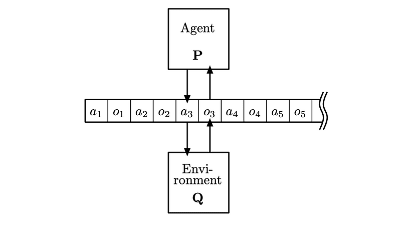
The action / perception loop has occupied the intellectual body of humanity since the times of ancient philosophy. The development of the so-called cybernetics and control-theory in the latest part of the last century revived the speculations with more mathematical form than just the philosophical investigations of the 17th century (Kant, Laplace, etc.).

To a cybernetician everything is a feedback loop and therefore action / perception should be studied through this prism. Two core principles behind active inference are coming from the early work of system modeling and cybernetics; namely Homeostasis and Good Regulator principle, both of which are part of other fields like biology and economics Some will argue that these fields are not truly scientific; however it is their complexity that make them highly speculative when no experiment can study the phenomenon. Conducting science under high uncertainty is both an art and a science.

The Good Regulator principle states that “every good regulator of a system must be a model of that system”. This is nothing fancier than just saying you need to be able to predict what your actions will do, in order to plan ahead. This is the model-based RL dogma stated 50 years ago.

Now let’s focus on Active Inference. An agent acts to minimize it’s future surprise according an internal model that predicts the future state of the world. Additionally, the agent updates the internal model after the agent has acted in the world and new experience is gathered. This continues ad infinitum and life goes on. Intuitively, this means that an agent changes the actions to influence the future observations or change the expectation about them, allowing two routes for minimization of the surprisal surprisal is to surprise what functional is to a function.; namely action and perception.

Minimizing surprise through planning and perception

Surprise mathematically can be described as the negative model evidence of the observations $\mathbb{E}[-\log p(X)]$. An interesting observation here is that $p()$ captures a subjective probability here; it is a belief maintained by the agent. In order to keep itself inside the space of the expected observations, the agent has the option either to update it’s belief about observations or select actions that won’t cause unexpected outcomes. This surprise minimization through action and planning is Active Inference.

Let’s slowly dive into this mathematically:

We start from the principle that we need to minimize the expected surprise $-\log p(x)$.

In Ortega et al. [?], the interaction of the agent with the environment is described as a conversation between the agent and its environment that interacts with. Imagine the world as a tape where an action is modifying the state of the world which in turn provides a new observation which is received from the agent.

Let’s unwrap this in a bit more detail. The main principle behind active inference is homeostasis. Homeostasis in systems theory is the idea that a system doesn’t deviate from its equilibrium. A deviation of the equilibrium translates to surprise for the agent. However, quantifying this surprise requires the agent to have access to the observation (to compare against the equilibrium point). However, since we’re talking about future observation, this is inaccessible and therefore we need to predict such future observations. An important take away here is that the equilibrium point forms a “desired” observation with respect to the constraints of the system (e.g. a physical system that minimizes energy). A goal to be achieved in that sense can become the equivalent of the potential energy that the agents seeks to minimize. Kinetic energy refers to the past (where I’m now is a function of my past) and the future direction is influenced by the potential energy.

During the course of this article, we will focus on the Partially Observable setting of Markov Decision Processes.

Subjective expected utility https://arxiv.org/pdf/1512.06789.pdf

Uncertainty and Bounded rationaly:

Uncertainty is the opposite of knowledge. If we accept that an agent acts according its subjective expected utility then uncertainty becomes the opposite of utility.

Example: Imagine you want to act to the world to protect yourself from the rain. Random variable $X$ is the observation of rain, $A$ is the action of getting an ombrela with you and $S$ is the state of the world that expresses itself as rain ($S$ captures the amount of water in the cloud). These random variables are subscripted by $t$ and past with future variables are differentiated by subscripts $\leq t$ and $>t$ respectively.

[ pretty visuals break and description of homeostasis ]

The loop is pretty simple and the key ingredients are the following:

• The agent maintains a generative model which correlates actions, observations and states.
• The agent then plans to minimize its future surprise according the generative model (action).
• Once the agent acts and collects new experiences, it updates the generative model to make new observation less surprising (perception).

Note: a generative model captures the correlations between it’s random variables factorized by the structure/dependencies between the random variables.

Before we dive into further let’s take a break to review Variational Inference. We want to estimate the posterior distribution $p(z|x)$, where $x$ is the observed variable and $z$ the latent variable which models the hidden cause of our observation (e.g. $z$ could be the parameters of a process). This is traditionally called inference. However, usually there are some intractable computations involved. Using Bayes rule we see that $p(z|x)=\frac{p(x|z)p(z)}{p(x)}$. The normalizing factor $p(x)=\int{p(x, z)dz}$ depends on the cardinality of $z$ which might be prohibitively large.

However, one could try to approximate $p(z|x)$ with a variational density $q(z)$ (usually called the recognition model). The desideratum in this case would be to minimize the KL divergence $D(q(z)||p(z|x))$. From the definition of KL divergence it follows that

The last part can be factored further as:

Finally, after we tidy things up, we get:

$p(x) - D(q(z)||p(z|x)) = \underbrace{\mathbb{E}_q[\log p(x|z)]}_{\text{accuracy}} - \underbrace{D[q(Z)|p(Z)]}_{\text{complexity}} \coloneqq \text{ELBO}$

As $p(x)$ doesn’t depend on $q$, maximizing the left-hand side has the effect of minimizing the distance of the approximate posterior $q$ and true posterior $p(z|x)$.

What that means is that for generative models that we don’t have a quick way for doing inference, a variational approximation of the posterior distribution can become easy to estimate by using common optimization techniques.

$\text{ELBO}$ is also called negative variational Free Energy and in Active Inference literature Free Energy name is usually preferred This is to signify the connection with statistical mechanics. . One important thing to note is that for Variational Inference to work, you need to specify a likelihood model $p(x|z)$ (how well are your data explained by $z$) and a prior over your latent variables $p(z)$ (subjective a priori knowledge over the hidden causes).

There is another view to think of the ELBO. The reconstruction error represents how well the recognition distribution $q(z)$ explains the data. Assigning more density on areas of the $Z$ space where the log-likelihood $\log p(x|Z)$ is high means we get to explain the observations better. However, explaining the observations come with an information processing cost. For example, a good choice of $q(z)$ would be to assign all the mass around points that maximize $p(x|z)$, however this is effectively memoization. Instead, we seek to avoid having high mutual information between $z$ and $x$ and therefore we penalize $q(z)$ for deviating from $p(z)$. This lagrangian formulation solves a multi-objective problem. Maximize the explainability of the data through $z$ while keeping $q(z)$ as wide as possible.

Generative density over states and observations $p(o,s)$ Variational density over states $q(s)$

Minimize the $-\log p(s)$.

Absorbing utility functions into prior beliefs. This is quite confusing point $p_{desired}$ might be better.

One way to see the recognition distribution is that it models the inverse of the likelihoods. By minimizing the variational Free Energy, the agent is bounding its surprise (negative log model evidence) which is the difference between the prior expectation and the actual observation.

For a gentle bit of formalism, this translates to the following.

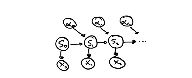
The generative model, $p(S,X,A)$ which is a joint over the actions $A$, states $S$ and observations $X$.

[ pretty visuals showing what the fuck ]

Breaking down the expected future free energy etc. and all this madness.

“The recognition model is the inverse of a likelihood model: it is a statistical mapping from observable consequences to hidden causes”

TODO [ ] Predictive coding - connection between prediction and compression [ ] Bounded Rationality - The cost of reducing uncertainty.